


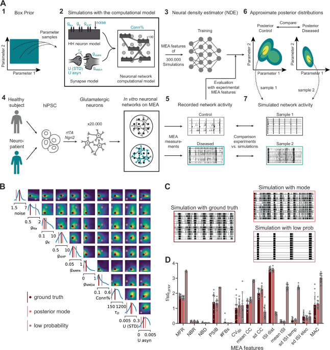
In vitro MEA data acquisition
We used data from neuronal networks derived from hiPSCs, previously cultured and recorded on MEA. hiPSC cells were differentiated into excitatory cortical Layer 2/3 neurons through doxycycline-inducible overexpression of Neurogenin 2 (Ngn2) as described previously1,2.
Informed consent was obtained from all subjects before using their hiPSCs, and approval was obtained from the medical ethical committee of Radboud University Medical Center, Nijmegen (2018-4525). All ethical regulations relevant to human research participants were followed.
The control line used for both pharmacological experiments and as control with diseased and gene-edited networks was obtained from the Coriell Institute (GM25256, RRID: CVCL_Y803) and was reprogrammed from skin fibroblasts of a 30-year-old healthy male. It was previously described and characterized3,41.
Drug manipulations were previously performed on neuronal networks derived from the control line as described in Doorn et al.11 for Dynasore and in Doorn et al.10 for MK-801, using the 24-well MEA system (Multichannel systems, MCS GmbH, Reutlingen, Germany), with a sampling frequency of 10 kHz.
MEA recordings of neuronal networks derived from patients with GEFS+ and DS were kindly provided by Nael Nadif Kasri and Eline van Hugte, and are described (Control, PAT001 GEFS, PAT001 DS) in van Hugte et al.7. Activity was recorded on the 24-well MEA system (Multichannel systems, MCS GmbH, Reutlingen, Germany) for 10 min with a sampling frequency of 10 kHz.
MEA recordings of control and CACNA1A+/− networks were kindly provided by Nael Nadif Kasri and Marina Hommersom, and are described in Hommersom et al.24. Activity was recorded on the Maestro Pro MEA system (Axion BioSystems, Atlanta, GA, USA) for 5 min with a sampling frequency of 12.5 kHz. Because this MEA system had 16 electrodes per well, we omitted the corner four electrodes from analysis, to mimic the electrode topology of the Multichannel MEA system and the computational model.
During all recordings, the temperature was maintained at 37 ∘C, and a flow of humidified gas (5% CO2 and 95% ambient air) was applied onto the MEA plate.
Computational model
The in silico computational model is described in Doorn et al.10, with the addition of asynchronous neurotransmitter release described in Doorn et al.11. In short, the model consists of one hundred Hodgkin-Huxley neurons with leaky channels and voltage-gated sodium and potassium channels. We also include sAHP channels, modeled as potassium channels whose conductance increases upon AP firing. The neurons are heterogeneously excitable through a variable constant external input current, accounting for intrinsic differences. In addition, we induce stochastic fluctuations of the membrane potential of neurons to mimic the effect of spontaneous neurotransmitter release or channel noise. Neurons are connected to a fraction of other neurons through synapses. These synapses include models of AMPArs, which open immediately upon arrival of a pre-synaptic spike and close rapidly. Additionally, we include NMDArs, which open and close slowly. The NMDArs are blocked by magnesium ions that are removed upon depolarization of the post-synaptic neuron. The strengths of the synapses vary slightly and are modulated by STD, following the Markram-Tsodyks model42.
Pre-synaptically, neurotransmitters are released synchronously (time-locked to the arrival of the AP), and asynchronously (where the release probability increases upon repetitive firing), following the Markram-Tsodyks model extension by Wang et al.43. Neurons were placed on a grid, allowing for the inclusion of distance-dependent conduction delays and virtual electrodes, mimicking MEA measurements.
To ensure computational feasibility and model interpretability, we fixed specific model parameters related to membrane and synaptic time constants while allowing others, such as ion channel conductances and synaptic strengths, to vary. The membrane time constant emerges from passive properties such as the membrane capacitance and leak conductance, both of which remain stable in most disease conditions44. AMPAr and NMDAr decay are fixed because they are determined by receptor subunit composition, which is developmentally regulated and remains stable under most pathological conditions45. Ion channel time constants are highly correlated with the expression of that ion channel14, so allowing both time constants and maximal conductances to vary would result in parameter redundancy and less interpretable posteriors. Therefore, we fixed time constants while keeping ion channel conductances free to vary. Lastly, Nernst potentials were fixed because they are mainly governed by astrocyte function. Since our cultures have healthy astrocytes, not patient-specific ones, we assume the astrocyte-related contributions to remain constant and unrelated to disease mechanisms. Fixed parameter values and prior ranges of the free parameters can be found in Table 1.
Forward simulations were performed using the Brian2 simulator46. One simulation took about two to three times the simulated time on a regular desktop CPU. To parallelize simulations across multiple desktop computers, we used a distributed computing method with dynamical load balancing47. While this platform significantly accelerates computation and facilitates flexible resource usage, it is not essential to the simulations themselves—similar performance could, in principle, be achieved with alternative parallel computing architectures.
Pre-processing and feature extraction
In vitro MEA recordings and in silico virtual electrode recordings are pre-processed and analyzed identically. Signals were filtered between 100 and 3500 Hz using a fifth-order Butterworth filter. We detected spikes using an amplitude threshold-based method, where the threshold was four times the root mean square of the electrode signal.
The computed MEA features are summarized in Table 2. The network firing rate was computed by binning spikes at all electrodes in 25 ms time bins. To detect NBs, we employed two thresholds on this network firing rate to start and stop the NB, set to 1/4th and 1/50th of the maximum firing rate respectively. Additionally, 50% of the active electrodes (i.e., electrodes with an average firing rate above 0.02 Hz) had to be firing during the NB, and the firing rate should remain above the NB start- or stop-threshold for 50 ms to start or end NB detection. To detect NB Fragments, we smoothed the network firing rate by convolution with a Gaussian kernel and used a peak detection algorithm on the smoothed network firing rate where peaks should have a minimal height of 1/16th of the maximum firing rate and a minimal prominence of 1/20th of the maximum firing rate. From this NB detection, we constructed five features. Specifically, we calculated the NB Rate (NBR), describing the number of NBs per minute, the NBD, describing the time between the start and stop of the NB in seconds, the Percentage of Spikes in NBs (PSIB), describing the percentage of spikes contained in the detected NBs, the number of fragments per NB (#FBs), and the coefficient of variation of the inter-NB-intervals (CVIBI).
We computed eight additional features describing other characteristics of the data. The first feature was the mean firing rate (MFR). Then we computed the continuous inter-spike-interval (ISI) time-series per MEA electrode, by determining the time between the previous and next detected AP for every time point. From these ISI-time-series, we computed the average ISI (mean ISI) across all timepoints and electrodes. By first taking the average ISI-time-series across electrodes, we defined the standard deviation of the ISI over time (sd ISI temp), and by first taking the average ISI across time points, we defined the standard deviation of the ISI over electrodes (sd ISI elec). Moreover, we computed the sample correlation coefficient between every pair of electrodes ISI-time-series. From this, we computed the average correlation coefficient (mean CC) and the standard deviation of the correlation coefficients (sd CC). Finally, we computed the average ISI-distance between every pair of electrodes as described in Kreuz et al.48. The above measures describe the spiking behavior of a network as well as the variation of spiking behavior temporally and spatially. Finally, to have a measure for the strength of oscillations in the network activity without relying on NB detection, we computed the Maximum Autocorrelation Component, as described in Maheswarenathan et al.34.
We trained the NDE on two additional features, the average and standard deviation of the correlation coefficient between binarized spike trains. However, we observed high correlations (0.96) between these features and the mean CC and sd CC of the ISI-time-series. Consequently, we chose not to show these features in the figures and we argue they could be omitted from training of the NDE.
Simulation-based-inference
To estimate the posterior distribution of the free parameters of the computational model, we employed amortized single-round neural posterior estimation17 using the SBI toolbox16 in a Python 3.9 environment. We sampled 300,000 parameter configurations from the prior distribution (a uniform distribution within the ranges shown in Table 1) and performed 3-min simulations with the computational model with each of these configurations. For every simulation, we computed the 13 MEA features described above. Next, we trained an NDE on these parameter configurations and resulting MEA features. This NDE was the standard Masked Autoregressive Flow provided by the SBI toolbox. Then, we evaluated the NDE with MEA features from either simulated network activity (for posterior-predictive checks) or experimental network activity. This resulted in a posterior distribution for each observation. Posterior distributions were visualized by plotting the marginals of 1000 samples drawn from the distribution.
As a check for the accuracy of the inference, we performed posterior-predictive checks. Initially, we used ground truth model parameters to generate simulations. The trained NDE was then used to estimate the posterior distribution of model parameters consistent with these simulations. The univariate and pairwise marginals were then inspected to see whether the ground truth model parameters fell within regions with a probability above 50% of the maximal probability. We performed posterior-predictive checks with NDEs trained on 100,000, 200,000, and 300,000 simulations, to see when the posterior distributions converged and checks were sufficient (all twenty-five checks in 50% or higher regions). To visualize the accuracy of the estimation, we performed ten simulations with the mode of the posterior distribution, the ground truth model parameters, and low-probability model parameters, and quantified the MEA features. For visualization, we normalized the MEA features by the standard deviation of that feature in the 300,000 simulation dataset. Additionally, we computed the Parameter Recovery Error (PRE) for each parameter for each of the twenty-five configurations, which is a measure of how concentrated the marginal is around the ground truth parameter value49.
Statistics and reproducibility
We compared MEA features of simulations generated with model parameters from the mode of the posterior distribution to MEA features of the corresponding experimental measurements. We performed statistical analysis using GraphPad Prism 5 (GraphPad Software, Inc., CA, USA). We first assessed the normality of the distributions using a Kolmogorov-Smirnov test. Given that normality of the features was often not ensured, we used non-parametric testing using a Mann-Whitney test to determine whether simulation and experimental features showed significant differences.
To investigate possible compensation mechanisms between model parameters, we generated 50 conditional distributions by holding all but two model parameters constant at values sampled from the posterior distribution and finding the distribution of the remaining pair of model parameters17. We then took 50 points from the resulting distribution and computed the Pearson correlation coefficient between the two model parameters, repeating this for every pair of model parameters. This resulted in 50 correlation coefficients per model parameter pair. To assess whether the average correlation coefficient per model parameter pair significantly differed from zero, we performed a one-sample t-test using GraphPad Prism 5. Normality was ensured using Shapiro-Wilk test.
To identify which parameter distributions were affected by drugs or disease, we compared the univariate marginals. First, we calculated the marginals using the MEA features of every network before and after drug application. We then took 50 samples from the marginals from each test and assessed whether the samples originated from different distributions using a Kolmogorov-Smirnov test using the Scipy stats package within a Python environment. This resulted in one P value per network. The number of networks is indicated in the figure captions. Dynasore networks were from two independent neuronal and astrocytic batches and MK-801 networks were from three independent neuronal and astrocytic batches. For comparison between healthy and diseased networks, we averaged the MEA features per cell line per MEA (different independent neuronal and astrocytic batches) and calculated the marginals. The number of batches is indicated in the figure captions. Using 50 samples from each set of marginals, we performed a Kolmogorov-Smirnov test, resulting in a p value per MEA.
Reporting summary
Further information on research design is available in the Nature Portfolio Reporting Summary linked to this article.
link