


In this work, we analyse a dataset we have collected between 2020 and 2024 that contains the temporal evolution of the network of personal relationships among 888 people belonging to the Blas de Otero High School in Madrid (see the “Methods” section for details on the data collection, data composition and data curation). The reported relationships were coded as +2 (very good), +1 (good), −1 (bad), and −2 (very bad). Almost every student provided this list, resulting in the extraction of a weighted directed network for the entire high school, which we will refer to as a snapshot or wave. We repeated this process every 16–20 weeks, and with this data, we reconstructed the network at different points in time, collecting 10 snapshots of the network over 4 years. With respect to previous literature, we have introduced some improvements in the data collection process. Respondents are allowed to report an unlimited number of relationships, resulting in richer and more heterogeneous data. We also increased the sample size by one order of magnitude, with a larger number of snapshots, allowing for the detailed study of the dynamics in the long term while maintaining a certain level of granularity. Relationships are self-reported, and they are directed and weighted, between −2 and 2, allowing the consideration of negative relationships. Preliminary analyses of earlier, shorter versions of this dataset have been reported elsewhere44,45. It is worth noting that by coding relationships into these four categories (−2, −1, +1, and +2), we inevitably lose many of the details that characterise social interactions. Real-world relationships exist on a spectrum, with layers of emotional, social, and contextual subtleties that cannot be completely captured in these discrete categories. Moreover, respondents may not report their relationships with the exact granularity imposed by our discretisation, as these relationships are inherently multifactorial and span multiple dimensions of variability. Thus, the resulting network we analyse in this study is not a direct reflection of the complexity of real personal relationships, but rather a simplified representation. Nevertheless, even with this simplification, we argue that identifying an equilibrium in the network serves as a meaningful proxy for the underlying dynamics of real social interactions. The equilibrium we detect in this reduced representation suggests that the macroscopic patterns of stability likely reflect deeper, robust social structures. Importantly, this simplification enables the mathematical rigour of our analysis; if equilibrium behaviour is clearly observable in the simplified model, it implies a genuine stability in the underlying network of relationships, even if the full complexity of these relationships is not entirely captured.
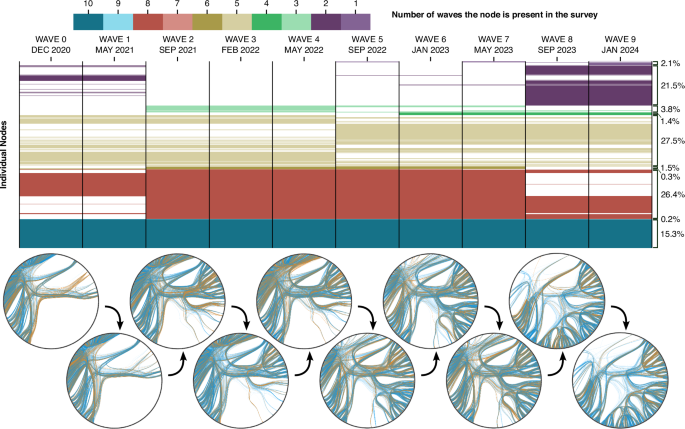
In total, we surveyed 888 people, but not all of them were present in all waves because the composition of the network changes as time goes by. We surveyed people belonging to a high school over the course of four academic years. Every academic year, new people enter the high school to take the first course, and at the end of the school year, almost all the people belonging to the last course leave the high school (a minor portion of them need to repeat the course if they fail their subjects). Thus, every academic year, some nodes appear in the network, and others disappear. In Fig. 1, we depict this turnover in a visual manner. Only 15% of the people are present in both the first and the last waves. This will become a very relevant fact when we show the network is in equilibrium, because this equilibrium will not result from the same group of people interacting over the course of four years, but rather an internal property of the network dynamics independent of the network composition. Due to this turnover, every snapshot of the network contains about 500 active nodes out of the 888. Let us define some notation for the discussions that follow. Throughout the paper, we will distinguish between a ‘link’ and an ‘edge’. Although these two concepts are often treated interchangeably, here we differentiate them. A link (or tie) refers to the directional connection from one node to another, whereas an edge represents the pair of links connecting two nodes (one in each direction). We provide a more detailed explanation of this distinction later in the manuscript.

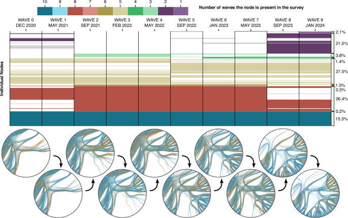
The table in the upper part shows the presence of individuals across the waves. Each row represents a person, and each column represents a wave. A coloured cell indicates the person’s presence in that specific wave. The cell colour reflects the total number of waves that the person participated in. Thus, all individuals present in n waves will have n cells coloured in the same colour, with a different colour for each n. Colours are not evenly distributed because each individual is likely present in all waves of the same academic year (dropouts or new enrolments in the middle of the year are rare). On the right side, the percentages of people present in each number n of waves are displayed. For instance, 15.3% of individuals are present in 10 waves, 0.2% in 9 waves, etc. Below the table, a visual representation of the evolution of the network of positive and negative relationships is shown. Individuals are represented as nodes arranged in a circular layout, with blue links for positive relationships and orange links for negative ones. To illustrate the high turnover in network composition, all individuals are depicted in every wave, even if they have not yet joined or have already left the network.
Stationarity of the transition matrices
In a nutshell, the concept of dynamical equilibrium in a physical system implies that the macroscopic, average properties of the system remain constant, fluctuating around a stable value, while microscopic dynamics are actively changing. For instance, in a gas, the microscopic components (the particles) are constantly moving at different velocities, colliding, vibrating, etc. However, if the gas is in equilibrium, macroscopic properties such as temperature, pressure, or volume remain constant.
Drawing an analogy to a social system represented as a network, it is essential to define both the macroscopic properties and the microscopic dynamics. In a social network evolving over time, links appear, disappear, or change in nature. From the perspective of a node, an outgoing or incoming +1 link can become a +2, a −1, a −2 or disappear. We refer to an absent link as a 0 link. This constitutes the microscopic dynamics of the system: the evolution of individual ties/links. From these microscopic components, we can build macroscopic properties of the network. In the network, we define an edge as the connection between two nodes that contains two links, one from the first node to the second and one from the second node to the first. Since we have 5 types of links, −2, −1, 0, +1, +2, there are 25 possible edge types. Notice the distinction between link/tie and edge that we introduce in our nomenclature. Although it is usual to treat both as interchangeable, we keep this distinction throughout the paper. Our first macroscopic property is the distribution of different edge types: how many +2+2, +1+2, +1+1, etc., edges exist in the network. Notice that a +2+1 edge is not equivalent to a +1+2, especially from a dynamical perspective. Although both edges can evolve towards a +1−1 edge, in the +2+1 case, the +2 needs to become a +1 and the +1 a −1, and in the +1+2 case, the +1 remains unchanged and the +2 becomes a −1. Therefore, we keep this distinction in all computations. A second macroscopic property is the in-degree and out-degree distributions of the nodes. For each type of link (+2, +1, −1, and −2), we count how many nodes have 0 incoming +2 links, 1 incoming +2 links, etc. This process is repeated for outgoing links and every type of link, generating eight-degree distributions. A third macroscopic property can be the distribution of different triangle types that can form among three nodes. Other macroscopic properties include structural characteristics of the network, such as clustering, average shortest path length, assortativity, centrality metrics, etc.
In this paper, we focus on the assessment of the degree, edge, and triangle distributions since we want to be able to define transition matrices to predict the expected equilibrium states of these macroscopic properties from the dynamics observed, ensuring the conclusions apply to all macroscopic properties. To assess whether our conclusions extend to more complex structures within the network, we have included an exemplary analysis of betweenness centrality and the details of this supplementary analysis are provided in the Supplementary Note 1. Before going into the details, it is important to comment on the limitations of our approach from the statistical mechanics point of view. The main challenge is the absence of a continuous concept of time in our analysis. By relying on snapshots taken every 20 weeks, we lose information about the transitions that occur between these intervals. Hence, there is an implicit assumption that no multiple transitions between edge states have occurred within the period between snapshots, minimising the risk of hidden dynamics. It is clear that this assumption may not hold in all cases: in systems like a gas, for example, relevant changes happen on much shorter time scales, making such large gaps between observations inappropriate. This point is important because there is a close relationship between the timescale of the network dynamics, the measurement intervals, and our ability to detect equilibrium behaviour. In networks with slower dynamics, transient fluctuations may persist longer and result in more frequent apparent violations of the equilibrium, as the system might not have enough time to relax back to equilibrium between observations. Conversely, if the network dynamics are too fast, although the equilibrium state may be accurately detected, the transition matrices might not fully capture the system’s internal dynamics because multiple transitions on the same link could occur between snapshots, distorting the measured change probabilities. However, in the context of social networks, the underlying dynamics evolve more slowly, and we believe that 20-week intervals provide a sufficient resolution. Besides, the use of statistical mechanical techniques in this study necessarily involves certain approximations to simplify the analysis of complex social systems. We aim at striking a balance between revealing meaningful sociological patterns and maintaining the rigour without becoming overly entangled in these mathematical details.
Let us introduce the concept of a transition matrix using the edges as our macroscopic property. We define the edges transition matrix mK as the matrix whose ij element represents P(j∣i), i.e., the conditional probability of an edge of going to the j state in one snapshot provided it started in the i state in the previous snapshot (see the “Methods” section for the construction of this matrix). The letter K labels the transition, such that mA is the transition between snapshots 0 and 1, mB is the transition between snapshots 1 and 2, etc. Additionally, we define the edge state distribution πt as a column vector in which each element i is the density of edges of type i in the snapshot t. With these two objects, it is clear to see that:
$${\pi }_{t+1}={({m}^{K})}^{T}{\pi }_{t}$$
(1)
In other words, if we take the distribution of edges in one snapshot and multiply this distribution by the transition matrix, we obtain the distribution of edges in the next snapshot. Since we have 10 snapshots, our data allows us to construct nine transition matrices between consecutive snapshots. The first relevant question is whether these nine transition matrices are statistically equivalent. If they were, it would indicate that the dynamics are stationary, meaning the transition probabilities between edge states remain constant over time. In the “Methods” section, we explain how to perform such a comparison.
Our findings show that the nine transition matrices are statistically equivalent (Fig. 2). We find that for transitions 1–9, the proportions of transitions with a p-value below our significance level (see the “Methods” section) are, respectively, 0.0016, 0.0112, 0.0128, 0.0224, 0.0176, 0.0096, 0.0096, 0.0096, and 0.0144. This indicates that, although some entries in the transition matrices deviate more than expected by chance, these deviations represent only a minimal fraction of the total transitions and can be attributed to normal fluctuations. All p-values and z-scores for the statistical comparisons are provided in the paper’s repository. Hence, we conclude that the stochastic process driving the network’s evolution is stationary, with constant probabilities governing the edge changes. Figure 2a.1–a.9 illustrates this with the individual transition matrices, and in panel (b) with the average transition matrix (see the “Methods” section for the construction of this average matrix), highlighting the similarity between them.

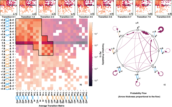
In (a.1)–(a.9), we depict the nine individual edge transition matrices, where each element ij represents P(j∣i). These matrices share axes and colour bar with (b), which contains the average transition matrix. In (b), we highlight a specific part of the average transition matrix. The highlighted transitions are those with more than 50 occurrences across the 10 waves. This threshold is arbitrary, chosen for visualisation purposes, but the entire matrix is included in all computations. In (c), we present a diagram illustrating the dynamics highlighted in (b). Specifically, we depict the selected edge types and use arrows to represent the probability flow between edge states, defined as P(i)P(j∣i). The arrow thickness is proportional to the probability flow. The self-loop of the + 0 + 0 edge is not depicted because it is disproportionately large due to the network’s low density. In this diagram, we have merged + 2 + 1 and + 1 + 2 links for simplicity of representation, although they are treated separately in computations; the same applies to + 2 + 0 vs. + 0 + 2, + 1 + 0 vs. + 0 + 1, etc. In a detailed representation, there should be two arrows connecting each pair of edges to represent the probability flow in both directions. However, as we will show, the detailed balance condition is fulfilled, which implies that the two flows are nearly symmetrical. Since our intention is to present a schematic illustration that simplifies the dynamic process for clarity and ease of visualisation, we use a single bidirectional arrow.
Given these results, it is natural to question whether the network is changing significantly. One might doubt whether the observed stability in dynamics is due to the network barely changing, with most edges remaining constant. For this reason, we included in Fig. 2c to illustrate the main dynamics within the network. While some edges are indeed stable, such as the + 2 + 2 edge, which is the most stable, there are still significant dynamics within these edges. Approximately half of the probability flow from this edge transitions to other states, showing that only a little over half of these edges persist from one wave to the next. For all other edges, the probability of transitioning to a different state is greater than that of remaining unchanged. This indicates that the dynamics are quite active, with a considerable turnover in edge states.
This strategy can also be applied to other macroscopic properties. For instance, at the level of triangles – similar to edges – we can identify all unique triangle states and construct a transition matrix for these states. Given that there are five different types of directed links, the number of combinations grows exponentially with the size of the macroscopic structures analysed. In the case of triangles, we identify 1924 unique triangles (the number we observe, not the theoretical maximum). Thus, we can construct a 1924 × 1924 transition matrix for triangles and perform a similar test. Similarly, we can apply this method to degrees. For each node, we have eight types of degrees (in and out degrees for +2, +1, -1, and -2 links). For example, for the +2 in-degree, we examine how many nodes with an initial +2 in-degree transition to a different +2 in-degree in the next wave. This allows us to construct a transition matrix for +2 in-degrees. Although the matrix size varies depending on the specific degree analysed, the strategy remains consistent. We stress that, in all cases, we find that the transition matrices governing the evolution of these macroscopic properties are stationary, indicating that the probabilities driving the network’s evolution are constant over time. In all three cases (edges, triangles, and degrees), we provide the abundances, transition matrices, z-scores, and p-values in the project’s repository as supplementary material.
Equilibrium state
The stationarity of the transition matrices does not necessarily imply that the network is in equilibrium; it may not even have an equilibrium state under these dynamics. As we will see, this is not our case.
Starting from equation (1), focusing on edges, we can determine whether the system has a stationary state under the dynamics governed by the transition matrix calculated. If it exists, we can calculate and compare it with the actual state of the network. In equation (1), we obtain the edge abundances in the next wave by multiplying the transpose of the transition matrix by the edge abundances in the current wave. When the system reaches the stationary state, these edge abundances become invariant under the transpose of the transition matrix. In other words, to find the stationary state associated with a transition matrix m governing the dynamics, we need to solve the following equation:
$$\tilde{\pi }={m}^{T}\tilde{\pi }$$
(2)
Here, \(\tilde{\pi }\) represents the stationary edge abundances, i.e., the edge abundances expected in the stationary state. Solving equation (2) is equivalent to finding the eigenvector of the transpose of the transition matrix associated with the eigenvalue 1. A comparable procedure can be applied to obtain the stationary abundances of triangles and the eight different degree distributions. Once we obtain these theoretical abundances of edges, triangles, and degrees expected in the stationary state under the system’s current dynamics, we can compare them with the current abundances to see where the system stands with respect to the stationary state. This comparison is depicted in Fig. 3.

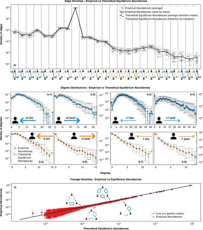
In (a), this comparison is depicted for the edges abundances, both the averages and wave by wave, while in the rest of the panels we depict only averages. In (b.1)–(b.8), this comparison is depicted for the eight different degree distributions. In (c), we depict the comparison for the triangle abundances. Since there are 1924 unique triangles spanning eight orders of magnitude, we have chosen a slightly different representation for the comparison. For each triangle motif, we plot the theoretical equilibrium abundances on the x-axis and the empirical abundances on the y-axis. Thus, each point corresponds to a theoretical-empirical pair for each motif, and the closer a point lies to the y = x line, the better the match between the two. For visualisation purposes, we have also included four exemplary motifs corresponding to some of the depicted points, chosen arbitrarily. In all cases, the error bars correspond to the 95% confidence intervals, and details for their computation are provided in the “Methods” section.
It is significant to note that in all cases, we find that the theoretical stationary states coincide with the observed empirical abundances, which indicates that the system has reached the stationary state. Nonetheless, to say that the system has reached the stationary state is not equivalent to saying that the system has reached the equilibrium. To rigorously claim that the system is in dynamical equilibrium in the statistical mechanical sense, we need to check that the Detailed Balance Condition is fulfilled. The Detailed Balance Condition ensures that a system has reached equilibrium and is expressed as46:
$$P(i)P(j| i)=P(j)P(i| j)$$
(3)
Where P(i) is the probability of the system being in state i, and P(j∣i) is the conditional probability of transitioning from state i to state j provided the system starts in state i. That is, this condition ensures that the probability flow for all transitions between every pair of states is equivalent in both directions. Using our notation:
$${({\pi }_{t})}_{i}{({m}^{K})}_{ij}={({\pi }_{t})}_{j}{({m}^{K})}_{ji}$$
(4)
Since both πt and mK are sampled from the data, there is some uncertainty associated with both sides of equation (4). Therefore, the Detailed Balance Condition needs to be fulfilled within the confidence intervals associated with both sides of the equation (see the “Methods” section for details and the project’s repository for the raw numerical results on these values and confidence intervals). We find that equation (4) is satisfied for almost every transition between edge states within the confidence intervals. We observe small violations of the Detailed Balance Condition in some transitions between edge states. A table summarising the characteristics of those transitions exhibiting a violation is provided in the Supplementary Table S1. Overall, the proportion of transitions that do not fulfil the condition is 0.003, 0.01, 0.04, 0.01, 0.023, 0.027, 0.004, 0.01, and 0.007 for transitions 1–9, respectively. In all cases, the magnitude of the violation is minor. Specifically, for the instances where a violation occurs, we have computed the z-scores, defined as the number of standard errors by which the condition is not met. In the majority of cases, the z-score is between 2 and 3, indicating that although the condition is not strictly fulfilled, it is very nearly so. Overall, given the low frequency and small magnitude of these violations, we conclude that they have a negligible effect on the equilibrium of the network. It is possible to detect in Fig. 3 the effect this violation has on the equilibrium abundances. For the edges and triangles affected, the equilibrium curves are slightly above the empirical abundances, although there is still an almost perfect overlap between both. The method’s ability to detect such a small violation supports the robustness of the equilibrium conditions found for the remaining transitions. The raw results for the assessment of the detailed balance condition for degrees a triangles are included in the project’s repository as well.
These observed violations might be attributed to simple statistical fluctuations in the network dynamics. Nonetheless, there appears to be a bias in the probability flows involved in these discrepancies, favouring the formation of new positive relationships. Although these fluctuations remain compatible with the equilibrium framework we present, it is worthwhile to explore the potential origins of these discrepancies. One plausible explanation is that these deviations may be linked to the fact that we analyse students during a critical developmental stage. During this period, individuals are likely enhancing their cognitive capacities and their ability to manage a larger number of social connections. Being this indeed the case, the equilibrium dynamics framework may be applicable only to short- and medium-term dynamics during these life stages. However, it is important to stress that this interpretation is speculative. The overall results align very closely with the network being in equilibrium, suggesting that, regardless of the underlying cause, these discrepancies have only a minimal effect on the network dynamics.
As a final complementary analysis, we examined whether a metric capturing more complex structural behaviour–specifically, Betweenness Centrality–exhibits a pattern similar to that observed for degrees, edges, and triangles. As we can see in Fig. 4, we observe that, in this case as well, the transition matrices are stationary, the detailed balance condition is fulfilled, and the empirical abundances coincide with the theoretical equilibrium distributions (see Supplementary Note 1 for all technical details). All raw numerical results are available in the project’s repository.

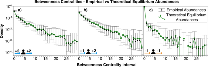
In (a), this comparison is depicted for the centrality measured considering only +2 links. In (b), this comparison is depicted for the centrality measured considering +2 and +1 links, treating them as equivalent. In (c), this comparison is depicted for the centrality measured considering only −1 links. The error bars correspond to the 95% confidence intervals, and details for their computation are provided in the “Methods” section.
link