


Traveling networks
We therefore introduce the concept of ‘traveling networks’—connected systems that change their location in space over time by rearranging their structure. This class of networks is motivated by various real-world systems, for example: (1) The slime mold Physarum polycephalum traverses the environment in search of food by rearranging its branched network (Fig. 1a, supplementary movie 1)21,22. (2) The subcellular actin cytoskeleton network drives eukaryotic cell movement through polymerization and depolymerization of its filaments (Fig. 1b)23,24,25. (3) Human corporations move through high-dimensional market spaces by creating new products and phasing out older ones (Fig. 1c)26,27,28,29,30. For each of these systems, a characteristic time scale τr exists after which none of their original structure remains and the network occupies a distinct new region of space (Fig. 1a–c). This makes these networks distinct from other well-studied networks that are able to dynamically grow and branch but do not leave their original rooted location7,9,10,11,12,13,14.

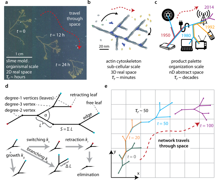
a–c Examples of traveling networks: a slime molds (2D real space)21, b actin cytoskelton (3D real space)23, c human organizations (high dimensional abstract space, depicting select products of Nokia Corporation over time)51,52,53. d Model of a traveling network based on an acyclic binary tree with two leaf types. ‘Free leaves’ (cyan) branch at rate kb, grow at rate kg, and switch at rate ks, to become ‘retracting leaves’ (red) which retract at rate kr until they reach a degree-three vertex. The branching angle is set by α, and the size of the network S is the sum of the edge lengths L. e The model from (d) results in a traveling network with conceptual similarity to (a–c). Time in arbitrary units. (a–c, e: Red arrow illustrates how networks travel through space; τr represents typical time scale after which the network has completely remodeled itself). (Image b inspired by23,54).
A traveling network model
This motivates a deeper investigation into the constraints and opportunities experienced by such traveling networks. Here we propose and analyze a tractable model (Fig. 1d) that involves a tree with maximum degree (number of edges connected to a vertex) of three (supplementary sections 2, 3). The leaves (degree-one vertices) are stochastically manipulated and can be in either a ‘free’ or a ‘retracting’ state. Free leaves undergo three possible manipulations: (1) growth by adding unit length ΔL at rate kg; (2) branching at rate kb, by creating two new free leaves—each with an edge of length ΔL at an angle ± α/2 from the previous edge, thereby converting the original leaf into a degree-three vertex; and (3) switching by becoming a retracting leaf at rate ks. Retracting leaves undergo only one manipulation: removing length ΔL at rate kr until they reach a degree-three vertex, upon which they are eliminated and generate a degree-two vertex. In this model, retracting leaves cannot switch back to being a free leaf. The amount of resources available to the system is represented by the overall size of the network, S, which is defined as the sum of all the edge lengths and implies that more spatially distant vertices require more resources to connect. S can be constant, or it can change over time depending on the system and external conditions. As the following analysis shows, the model’s restructuring rules lead to networks that exhibit characteristic dynamic structures (supplementary section 4), that travel through space (supplementary sections 5, Fig. 1e, supplementary movie 2), and that effectively search this space (supplementary sections 6). This model clearly neglects many aspects of any particular real system (Fig. 1a–c), yet it proves to be very informative for analyzing many key properties and behaviors of general importance to traveling networks.
Network structure and criticality
We first systematically analyzed the network structure and dynamics (supplementary section 4). The network structure is characterized by the number of each of the different vertex types and their connectivity and can be crucial to network performance. We focused on the case where the network size S is constant, which implies that kb = ks. We considered a representation that is based on rates that are normalized by kr (i.e., KB ≔ kb/kr, KG ≔ kg/kr, Ks = ks/kr, supplementary section 4.5.1). This allowed us to analyze the structure and behavior for networks of a given size in a phase space that is determined by just two independent restructuring parameters, i.e., KB ≔ kb/kr, KG ≔ kg/kr.
To visualize the network and confirm analytical results, we implemented a stochastic simulation embedded in 2D space (methods, supplementary section 8), though much of our analysis generalizes to higher spatial dimensions. We set kb = ks, and we numerically imposed preservation of size S by dynamically modifying the likelihood of switching up or down as needed (methods, supplementary section 8.1). We found that arbitrary starting configurations converge to steady state dynamics in which branching, growing, and retracting leaves cause the network to travel through space (supplementary movie 2). The observed network structures vary characteristically with KB and KG as indicated by the number of retracting (NR), free (NF), and total (N1 = NF + NR) leaves (Fig. 2a–d, supplementary movie 3); networks with high KB have more retracting leaves; if both KG and KB are small, most leaves are free, and a large ratio of KG : KB results in longer edges, fewer vertices, and fewer total leaves.

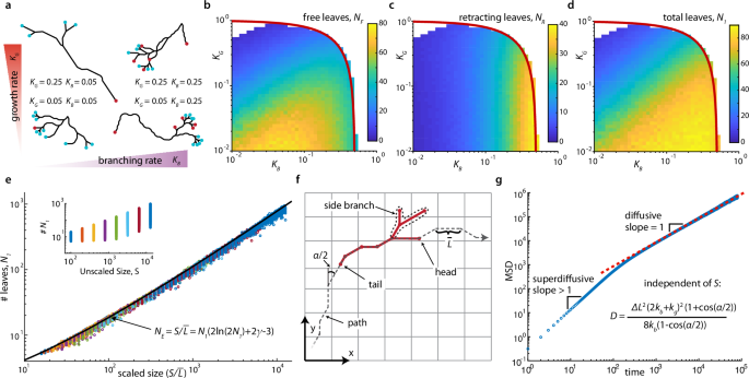
a A range of network structures are possible, illustrated by four typical networks at high/low KB/KG having different edge lengths, numbers of free leaves (cyan) and retracting leaves (red), and leaf type ratios (simulation of model from Fig. 1d; size, S = 70, supplementary movie 3). b–d KB and KG regulate the structure, exhibited by the mean numbers of free leaves (b), retracting leaves (c), and the total leaves (d) (simulated networks of S = 800; red lines: 2KB + KG ≤ 1 boundary of possible steady state behavior). e Total leaves, N1, for various sizes, S, across the steady-state parameter space of KB and KG shown in (b–d). Number of leaves depends primarily on the average branch length \(\bar{L}\) as captured by the relation \(S={N}_{1}(2\ln (2{N}_{1})+2\gamma -3)\), where γ is the Euler-Mascheroni constant (black line). Inset: N1 does not collapse with unscaled S. f The longer term network movement reveals a ‘tail’ and, in retrospect, a unique ‘path’, and a ‘head’ (supplementary movie 4). g The network (center of mass) moves superdiffusively over short time scales and diffusively over long time scales, with the diffusivity, D, set by kb, kg, ΔL, and α. kb = 0.2, kg = 0.1, α = 60, S = 200 shown here; red dashed line indicates analytical result.
We then derived a set of analytical relationships between the model parameters that ultimately fully describe the network structure (supplementary sections 4.1–4.4), and we confirmed these relationships with simulations (methods, supplementary section 8). The edge lengths are distributed geometrically with mean length, \(\bar{L}=\Delta L(1+\frac{{K}_{G}}{2{K}_{B}})=\Delta L\frac{2{K}_{B}+{K}_{G}}{2{K}_{B}}\). The number of all edges is NE = N1 + N2 + N3 − 1 (where Ni is the number of vertices of degree i), with N3 = N1 − 2 and N2 = NE + 3 − 2N1, and on average \({N}_{E}=S/\bar{L}\). The ratio of the number of retracting to free leaves is \({N}_{R}/{N}_{F}=R=2{K}_{B}+{K}_{G}=2{K}_{B}\bar{L}\). By analyzing a recursive limit case, we found the final determining formula \(S\approx {N}_{1}(2\ln (2{N}_{1})+2\gamma -3)\) (γ is the Euler-Mascheroni constant), which is in good agreement with simulations over the entire tested parameter space (Fig. 2e, supplementary section 4.4). The branching angle α (Fig. 1d) influences the embedding of the network in space but not the number of each vertex type or edge length distribution; embedding in higher dimensions leads to additional branching angles. Ultimately, the variables \(\bar{L}\), R, N1, N2, N3, NF, NR, and NE are fully determined by just the three parameters KG, KB, and S, with \(\bar{L}\) and R even being independent of the network size S.
We note that the model can be fully non-dimensionalized using both the relevant time and length scales, not just kr as above (supplementary section 4.5). This leads to just two independent parameters, i.e., the rescaled branching rate \({K}_{{B}^{*}}:=\frac{{k}_{b}\bar{L}}{{k}_{r}\Delta L}=\frac{2{k}_{b}+{k}_{g}}{2{k}_{r}}\), and the total number of edges \({N}_{E}=S/\bar{L}\). Hence in case only networks of a given constant size S are considered, this even reduces to a single independent parameter. (The branching angle α could be considered an additional parameter, but again only plays a role when embedding the network in space) All networks sharing these two parameters then belong to the same ‘universal form’ and show equivalent rescaled behavior (supplementary section 4.6). Since many real-world systems likely have more direct control over their specific rates than over NE and \({K}_{{B}^{*}}\), we instead focus our remaining analysis on the earlier representation that is based on network size S and the original rates (kb, kg, kr) or rates non-dimensionalized by kr (KB ≔ kb/kr, KG ≔ kg/kr).
Importantly, we also found that these networks belong to a class of systems that automatically self-organize to operate at a critical point31. Size preservation and steady state require that the network remain balanced between exponentially increasing and exponentially decreasing the number of free leaves (kb = ks, supplementary section 4), reminiscent of a critical Galton-Watson process32. In the case of fast retraction, (kr ≫ kb), the model exhibits features of self-organized criticality (SOC)31 with branching and retraction corresponding to slow driving and rapid relaxations (‘avalanches’), respectively (supplementary section 4.4.7). Utilizing the Riemann Zeta function, we found that the probability P(LR) of a retraction event of length LR is scale-free, following the power law \(P({L}_{R})=c{L}_{R}^{a}\), with c ≈ 0.74 and a ≈ −2.48 (supplementary section 4.4.7). Additionally, the network exhibits an approximately self-similar, fractal-like structure, which can be understood through the critical recursive dynamics by which the network travels and self-renews (supplementary section 4.4.8).
Network restructuring and traveling
Next, we analyzed how the network actually travels through space due to its branching, growing, retracting, and eventually disappearing leaves (supplementary section 5). One fundamental quantity for traveling networks is their relocation time, τr, the time it takes for the entire network to reorganize such that it occupies a new spatial position and none of its initial edges exist anymore (Fig. 1a–c, e). Interestingly, we find that the relocation time depends only on the number of leaves and branching rate \({\tau }_{r}\approx \frac{{N}_{1}}{2{k}_{b}}\) (supplementary section 5.4). Another fundamental aspect is a description of the network’s longer-term movement. In this acyclic model, for times larger than τr, we find that a single unique path exists that connects the network’s initial and final positions (gray dashed line in Fig. 2f, supplementary movie 4). We define the ‘tail’ vertex as the oldest vertex in the network. The tail follows this unique path on the network’s trailing end, advancing at rate kr and intermittently pausing whenever it reaches a degree-three vertex. We also define a ‘head’ (which can only be identified in retrospect) as the free leaf that moved along this path at the leading edge of the network never switching or retracting. The head advances with speed vh = ΔL(2kb + kg). To maintain a steady state length between head and tail along the path, 2kb + kg = f ⋅ kr must hold, where f ≤ 1 is the fraction of time the tail is retracting rather than paused. In the framework nondimensionalized by kr, this implies 2KB + KG ≤ 1, which constrains allowable values of KB and KG for steady state dynamics (red lines in Fig. 2b–d). Hence this type of network behaves like a chain of vertices moving along a random path while extending and retracting temporary side branches.
Focusing on the head dynamics, we identified a correlated random walk, which, over longer time scales, also corresponds to the motion of the network’s center of mass. This random walk has step size \(\bar{L}\), step rate 2kb, and turning angle α/2. The diffusivity of the head and correspondingly the entire network can be written entirely in terms of the fundamental parameters as \(D=\frac{\Delta {L}^{2}{(2{k}_{b}+{k}_{g})}^{2}(1+\cos (\alpha /2))}{8{k}_{b}(1-\cos (\alpha /2))}\) (Fig. 2g), which corresponds to the freely rotating chain model in polymer physics33,34. Interestingly, D is independent of network size. Networks with high kg and low kb diffuse fast (large D) but have structures with few free leaves (Fig. 2b). Having a small number of free leaves might be considered a risky configuration since it limits options for future directions of travel, and stochastic elimination of all free leaves at once could lead to catastrophic collapse of the entire network (methods, supplementary section 8). Together, the expressions derived above provide quantitative insights into the network’s structure and motion, moreover, since the same rates simultaneously impact both structure and motion, this analysis highlights how traveling networks face inherent tradeoffs.
Passive spatial search
Such tradeoffs become particularly important for spatial search, a task that many traveling networks perform in real or abstract spaces (Fig. 1a–c, supplementary section 6.1). We therefore analyzed the efficacy of random search for different target sizes by counting all unique boxes of different sizes35 that a network occupied within a given time period (Fig. 3a). We ran corresponding simulations on four networks with different combinations of high and low KB and KG (Fig. 3b). The low KB, high KG network collected the most large boxes, which can be understood through the expression for D, which indicates larger diffusivity for large KG. Networks with higher KB collected the most small boxes since new lengths of \(\bar{L}\) are added at rate NF ⋅ 2kb (before the network begins crossing itself). The low KB, low KG network diffuses slowly and does not add much length per time hence it is not an effective searcher at any length scale. Data from all four networks actually collapse to a single curve when rescaled, corresponding to the universal form discussed earlier (Fig. 3b inset, supplementary sections 4.6 and 6.1). The absolute value of the slope of these plots is the Hausdorff dimension of the network history which increases toward 2 with long runtimes as self-crossing becomes more frequent (supplementary section 6.1.4), consistent with Brownian trails in two or more dimensions35. Hence traveling networks can tune their restructuring rates for optimal multiscale search depending on the relevant time and length scales.

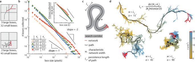
a Schematic of box counting quantification over time illustrated for two different networks with different search efficacy at different spatial resolutions (gray is the full past history, and red is final network position). b Four networks, S = 100, runtime: Δt = 2000, KB = (0.01, 0.3), KG = (0.01, 0.3) show that having low kb and high kg maximizes diffusivity and collection of large boxes (red diamonds), and high kb optimizes for collecting small boxes (blue squares and green triangles), illustrating a tradeoff between coarse and fine search. Low kb and low kg (peach stars) have worse performance across all sizes. (The slopes of −1 and −2 are inserted for visual guidance). Inset: Rescaling box size by \(\bar{L}\) and boxes collected by Nf ⋅ 2kb ⋅ Δt (the total expected \(\bar{L}\) units added) collapses this data onto a single curve. c Characteristic length scales of traveling networks include the network width, w, and path persistence length, Lp (supplementary sections 5.2.1 and 6.1.1). d Example networks of different w and Lp generated by varying branching angle, α (15, 45, 90 degrees) at constant S = 200, kb = 0.01, kg = 0, kr = 1, Δt = 20,000. The most recently occupied historic network positions fade from blue (recent) to gold (old); red is the final position, and black indicates the path. For w < Lp, the network sweeps a search corridor along its path, and for w > Lp the network behaves as a jittering blob.
Network size and branching angle affect how much space the side branches can explore, thus we analyzed how these parameters impact search behavior. Using the above expressions and understanding of the network’s structure and motion, we find that the path has a characteristic persistence length, \({L}_{p}=-\bar{L}/\ln (\cos (\alpha /2))\), and the network has a characteristic search width, w, (Fig. 3c) which itself has a more complex dependence on \(\bar{L}\), α, and S (supplementary section 6.1.1). For w < < Lp the network behaves like a particle sweeping a corridor, and for w > > Lp the network behaves like a jittering blob conducting a fine-scale search of limited scope, reminiscent of tradeoffs in depth-first and breadth-first search strategies36. This ‘search morphology’ is sensitive to α as illustrated in Fig. 3d. Counting boxes of size \(\bar{L}=1\) over time reveals that the optimal angle for search depends on the search duration, with w ≈ Lp collecting more boxes over shorter times and w < Lp collecting more boxes over longer times in these examples (supplementary section 6.1.5).
Active and biased spatial search
Beyond the random restructuring and motion considered so far, we now consider traveling networks that respond to their environments through biased restructuring (supplementary section 6.2). We extended the model by making the free leaves sense and respond to variations in the environment. Here the switching rate of every free leaf increases or decreases depending on whether the environment, represented by a scalar field, at that leaf’s position is smaller or larger, respectively, compared to the field averaged across all free leaves. This leads to a biased motion of the network up a field gradient (Fig. 4a, supplementary movie 5, methods, supplementary section 8.4.1). To capture environmental resource consumption as caused by natural systems (Fig. 1a)21,22, we coupled the network position to modifications of the field itself, leading to the network’s biased motion through a changing environment (Fig. 4b, supplementary movie 6).

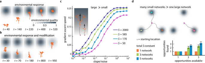
a, b Traveling networks can perform biased search by making leaf switching rates depend on the local vs. globally sensed environment in a stationary gradient (a) or even while modifying their environment (b). c When ascending noisy gradients, large networks tolerate lower slope-to-noise-ratios and ascend faster than small networks. Different network sizes: S, α = 60°, kb = 0.1, kg = 0. d Multiple small networks exploit more opportunities in environments with multiple opportunities than a single large network of the same total size. (n = 40 trials, error bars are one standard deviation).
Many other model alterations can capture various environmental responses. For example, in an alternative model we modified the rates based on only local information and allowed the network’s size S (which was kept constant until now) to change in response to a dynamic environment (supplementary movie 7, methods, supplementary section 8.4.2). This is akin to a physarum network (Fig. 1a) that moves in response to food in the environment, changes its network size accordingly, and modifies the food distribution in the environment by consumption21. A deeper and more systematic analysis of such networks is left for future work (supplementary section 7.2).
Importantly, these traveling networks can function as highly sensitive detectors as network size preservation self-organizes37 (or ‘self-tunes’38) them to operate at a critical point where small environmentally-induced changes to their fundamental underlying restructuring rates can cause enormous changes to their emergent structure and motion through local exponential growth and decay (supplementary section 6.2). Note that even when network size is not preserved, such critical behavior and thereby sensitivity could be implemented locally within subsets of the network.
Many real-world traveling networks (Fig. 1a–c) can split into multiple smaller entities or merge into larger structures (Fig. 1a, c)21,39, suggesting that trade-offs exist between network size and network number for performing efficient search tasks. We tested this hypothesis with simulations (Fig. 4c, d). We found that for responsive networks moving up a linear, noisy gradient, larger networks are able to move faster and tolerate higher noise levels than smaller networks (Fig. 4c). However, in a landscape with different numbers of ‘opportunities’, represented by local Gaussian maxima, multiple small networks are able to capture more opportunities than a single large network of the same total size (Fig. 4d, supplementary movie 8). Hence it can be more advantageous to allocate the resources into one large network or into multiple smaller networks – depending on the specific environment and search task.
Application to real-world systems
Connecting the traveling network concept and our analysis results back to our motivating examples (Fig. 1a–c), we note that evidence for similar connections between underlying parameters choices, network structure, and strategic movements exists in the literature (Fig. 5a–c). (1) Takamatsu et al.10 experimentally observed that Physarum adopts different network structures depending on its environment. More highly branched sheet-like networks formed under favorable nutrient-rich conditions contrasting with longer, spindly networks that formed in adverse chemical environments (Fig. 5a) (supplementary movies 7 and 9). (2) The actin literature connects (de-) polymerization and branching rates to cytoskelatal structure and movement, which then affect the number of filopodia and higher-level (search) behaviors of cells (Fig. 5b)24,40. There is also experimental evidence for SOC in actin networks41 similar to our model predictions (supplementary section 4.4). (3) The business strategy literature identified a positive correlation between shareholder returns and capital reallocation among a company’s business units (Fig. 5c)42,43, suggesting that active movement through the space of market opportunities via dynamic changes (termed ‘seeding’, ‘nurturing’ and ‘pruning’) is important for productivity. Additionally, there is also analysis of which factors make it advantageous for companies to merge or split (compare to Fig. 4c, d)44,45. In the context of a traveling network model, we identify how rates (kb, kg, kr) should be changed in order to select the desired behavioral strategy (Fig. 5a–c). Conclusions from the model analyzed here can be summarized in a concise 2D parameter space (Fig. 5d) (supplementary sections 4.5.2 and 4.6) that reveals various trade-offs, such as between coarse fast search vs. fine slow search or when switching between ‘exploration and exploitation’46 or when avoiding the risk of catastrophic collapse by operating sufficiently far away from non-steady state conditions at the expense of slower dynamics overall (red line, Fig. 5d).

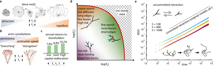
a Different Physarum network morphologies are seen in adverse and favorable environments (right vs. left)10. b Changes in actin cytoskeleton structure and resulting cell movement due to network restructuring by branching and elongation40. c Positive association between more capital reallocation (higher restructuring rates) and returns for corporations, 1990–2005, based on three quantiles of n = 1616 companies42. (Images in (a–c) adapted from the corresponding references. Up and down arrows indicate how restructuring rates might be changed within a traveling network model to achieve the behaviors; rate changes deduced qualitatively from the literature10,40,42,43. d Summary of behavioral and ecologically relevant network properties and their codependence on the underlying restructuring rates in a concise 2D parameter space (example network morphologies superimposed, overall conclusions independent of S; colors of vertices as in Fig. 1d, time nondimensionalized by kr). e A traveling network model without persistent retraction (‘uncommitted retraction’ model) explores the space more slowly than the original model (Fig. 1d), and becomes even less efficient with increasing network size.
Alternative models
So far, our analysis focused on one model with particular assumptions (Fig. 1d), but many real-world traveling networks likely follow very different restructuring rules. As a contrasting example, we analyzed a similar model in which retracting leaves were also allowed to revert back into being growing and branching leaves. Hence in this altered model only one leaf type exists, and leaves frequently alternate back and forth between retraction and growth (Fig. 5e). We found that for such an ‘uncommitted retraction’ model the resulting networks do not display the range of morphologies seen in Fig. 2a; instead these networks degenerate into a single chain of nearly unbranched degree-two vertices (Fig. 5e inset, supplementary section 7.1, supplementary movie 10). Furthermore, the diffusion rate significantly slows with increasing network size S, unlike the much faster and size-independent diffusion of the original model (Figs. 2g and 5e). Hence the ‘stay committed to retraction once started’ rule appears important here for achieving structural complexity as well as for effective motion and search, and, more broadly, rules as well as rates can have a profound impact on traveling network performance.
link